2023-HGU-ML Lecture 6. Decision Theory
Decision Theory
- given an input vector, our goal is to predict a corresponding target value
- The target value is described probabilistically
- DT provides optimal decisions in situations involving uncertainty, combined with probability theory
- Three approaches to making a decision
- generative model, \(p(t, x)\) or \(p(x \mid t)\)
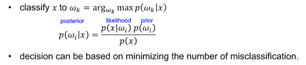
- can be used for the classification using \(p(t \mid x)\) = \(\frac { p(x \mid t)p(t) }{p(x)}\)
- generate new data or detect outliers
- Discriminative Model
- \(p(t \mid x)\), just classficiation
- Discriminant function
- f(x), model a map function from input x to a label t
- generative model, \(p(t, x)\) or \(p(x \mid t)\)
- probability models for decision
- misclassification rate vs. loss function
-
Type 1 and 2 error
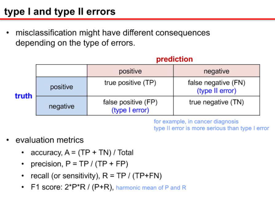
-
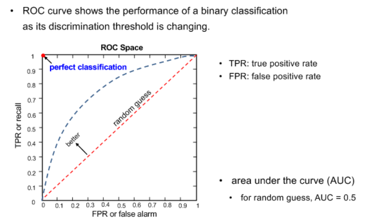
receiver operating characteristics (ROC)
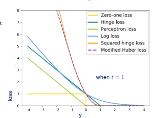
- loss function
- a function that maps an event onto a “cost” value
- minimum expected loss
- our goal is to minimize an expected loss (or risk)
- classify x into class which minimizes the conditional risk (or expected loss)
-
loss functions in general
- The term “probability” refers to the possibility of something happening. The term Likelihood refers to the process of determining the best data distribution given a specific situation in the data. When calculating the probability of a given outcome, you assume the model’s parameters are reliable.
- Three decision rules based on probability
- Maximum Likelihood
- Maximum a posterior
- Bayes Risk
Bayes Risk is a concept in decision theory that measures the expected loss associated with a decision, taking into account the uncertainty in the underlying parameters or states. It is derived from Bayesian decision theory, which combines prior knowledge with observed data to make optimal decisions.
In the context of decision theory, the Bayes Risk \((R(\delta))\) associated with a decision rule \((\delta)\) is defined as the expected value of the loss function under the posterior distribution of the parameters, given the observed data. Mathematically, it can be expressed as:
\[R(\delta) = \int L(\theta, \delta(x)) \cdot f(\theta | x) \, d\theta\]where:
- \(L(\theta, \delta(x))\) is the loss function, representing the cost associated with making a decision \(\delta(x)\) when the true state is \(\theta\).
- \(f(\theta \mid x)\) is the posterior distribution of the parameters given the observed data \((x)\) .
The Bayes Risk accounts for the uncertainty in parameter estimation by integrating the loss over the entire parameter space, weighted by the posterior distribution. This approach reflects the Bayesian philosophy of updating beliefs based on both prior knowledge and observed evidence.
In practice, the decision rule \((\delta)\) can be chosen to minimize the Bayes Risk, resulting in a decision that is optimal in terms of expected loss. The Bayes Risk provides a comprehensive measure of the cost associated with decisions, considering the uncertainty inherent in parameter estimation in a Bayesian framework.
Maximum Likelihood Estimation (MLE) and Maximum A Posteriori (MAP) estimation are both methods used to estimate the parameters of a statistical model, but they differ in their underlying principles and assumptions.
Maximum Likelihood Estimation (MLE):
- Objective: MLE aims to find the values of the model parameters that maximize the likelihood function, which measures how well the observed data is explained by the model.
- Assumption: MLE assumes a uniform or non-informative prior distribution, meaning that all parameter values are equally likely before observing the data.
-
Formula: \(\hat{\theta}_{\text{MLE}} = \arg\max_{\theta} \mathcal{L}(\theta \mid \text{data}),\) where $\mathcal{L}(\theta \mid \text{data})$ is the likelihood function.
- Result: MLE provides a point estimate of the parameters that maximizes the likelihood of the observed data.
Maximum A Posteriori (MAP) Estimation:
- Objective: MAP estimation combines the likelihood function with a prior distribution to find the values of the parameters that maximize the posterior distribution.
- Assumption: MAP incorporates prior knowledge or beliefs about the parameters by introducing a prior distribution. This prior reflects any information available before observing the data.
- Formula: \(\hat{\theta}_{\text{MAP}} = \arg\max_{\theta} P(\theta \mid \text{data}),\) where $P(\theta \mid \text{data})$ is the posterior distribution.
- Result: MAP provides a point estimate of the parameters that maximizes the posterior distribution, considering both the likelihood and the prior.
Key Differences:
- Incorporating Prior Information: The major distinction lies in the incorporation of prior information. MLE assumes a non-informative prior (flat prior), while MAP explicitly considers a prior distribution that may encode prior beliefs or knowledge about the parameters.
- Formula: The formulas for MLE and MAP are similar, but MAP includes the prior term in the optimization process, affecting the final estimate.
- Robustness: MAP estimates may be more robust when dealing with limited data because the prior helps regularize the estimation. MLE can be sensitive to sparse or noisy data.
In summary, MLE and MAP are both methods for estimating parameters, with MLE relying solely on the likelihood function and MAP incorporating prior information through a prior distribution. The choice between them depends on the available information and the desired balance between data-driven estimates and prior beliefs.
-
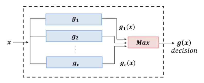
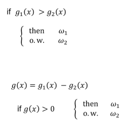
discriminant function g(x) using gi(x) (e.g., ML, MAP, Bayes risk)
-
decision boundary
- boundaries for Gaussian
- case1: features are uncorrelated (i.e., independent) with the same variance
- case2: the classes have identical covariance matrices
- case3: each class has a different covariance matrix
- https://www.cs.cmu.edu/~aarti/Class/10315_Fall19/lecs/Lecture3.pdf
- boundaries for Gaussian