2023-HGU-ML Lecture 8. Dimension Reduction
Dimension Reduction
- Many features
- provide more information and potentially high accuracy
- make it harder to train a classifier (the curse of dimensionality)
- increase the possibility of overfitting
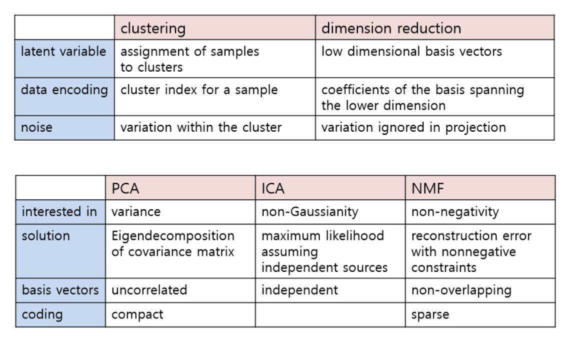
- principal component analysis (PCA)
- is one of the most popular and simple DR methods.
- is a linear projection
- finds an orthogonal basis set that makes the largest possible variance on the linearly projected space
- minimal reconstruction error``
- maximizing preserved variance after projection
- eigendecomposition of covariance matrix
- Rayleigh Quotient
- eigenfaces
-
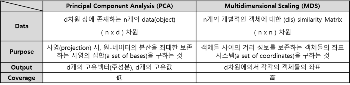
multidimensional scaling (MDS)
Multidimensional Scaling (MDS) is a technique used in statistics and data analysis to visualize the similarity or dissimilarity of data points in a high-dimensional space by projecting them into a lower-dimensional space. The goal of MDS is to represent the pairwise dissimilarities or distances between data points in a way that preserves the original relationships as much as possible.
Here are the key concepts and steps involved in multidimensional scaling:
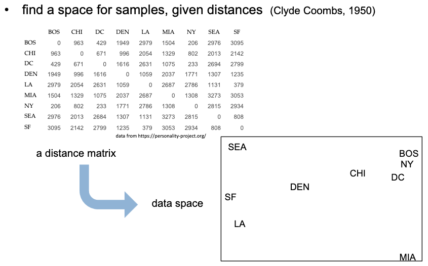
- Dissimilarity (or Distance) Matrix:
- MDS begins with a dissimilarity matrix, which contains the pairwise distances or dissimilarities between each pair of data points. These dissimilarities could represent any measure of dissimilarity, such as Euclidean distance, correlation, or other distance metrics depending on the nature of the data.
- Projection into Lower-Dimensional Space:
- MDS aims to find a configuration of points in a lower-dimensional space (typically 2D or 3D) such that the pairwise distances in the lower-dimensional space approximate the original dissimilarity matrix as closely as possible.
- Stress Optimization:
- The quality of the representation is often assessed using a stress criterion, which measures how well the lower-dimensional distances approximate the original dissimilarities. The goal is to minimize stress, indicating a good fit between the original and the lower-dimensional representation.
- Metric vs. Non-metric MDS:
- MDS can be classified into metric and non-metric MDS. Metric MDS preserves the actual distances between points, while non-metric MDS only preserves the order of distances (i.e., the ranking of dissimilarities).
- Applications:
- MDS is widely used in various fields, including psychology, marketing, geography, and bioinformatics. It is often applied to explore and visualize relationships between objects, such as similarity between products based on consumer preferences, geographic relationships between cities, or genetic similarities between species.
- Classical vs. Non-classical MDS:
- Classical MDS is based on eigenvalue decomposition and is suitable for metric MDS. Non-classical MDS, including methods like Sammon mapping, is used for non-metric MDS and often employs optimization algorithms to find the lower-dimensional representation.
In summary, multidimensional scaling is a valuable technique for visualizing and interpreting the relationships between data points based on their dissimilarities. It is particularly useful when dealing with high-dimensional data, as it provides a lower-dimensional representation that retains important structural information about the original data.
- Dissimilarity (or Distance) Matrix:
- non-metric pairwise data
- in the real world, many relations are asymmetric
- kernel matrix from asymmetric relations is not PSD
- PCA with inner products
- principle components regression (PCR)
- instead of regressing y (the dependent variable) on x directly, the principal components (PCs) of x are used as regressors.
- PCR regularizes the model (by using a subset of components)
- In statistics, principal component regression (PCR) is a regression analysis technique that is based on principal component analysis (PCA). More specifically, PCR is used for estimating the unknown regression coefficients in a standard linear regression model.
- In PCR, instead of regressing the dependent variable on the explanatory variables directly, the principal components of the explanatory variables are used as regressors. One typically uses only a subset of all the principal components for regression, making PCR a kind of regularized procedure and also a type of shrinkage estimator.
- https://deep-learning-study.tistory.com/668
- 통계에서 주성분 회귀(Principal Component Regression, PCR)는 주성분 분석(Principal Component Analysis, PCA)을 기반으로 한 회귀 분석 기법입니다. 보다 구체적으로, PCR은 표준 선형 회귀 모델에서 알려지지 않은 회귀 계수를 추정하는 데 사용됩니다. PCR은 설명 변수의 종속 변수를 직접 회귀하는 대신 회귀 변수로 설명 변수의 주성분을 사용합니다. PCR은 일종의 정규화 절차이자 일종의 수축 추정기이기도 합니다. 일반적으로 모든 주성분의 하위 집합만 회귀에 사용되기 때문입니다. 종종 분산이 더 높은 주성분(설명 변수의 샘플 분산-공분산 행렬의 더 높은 고유값에 해당하는 고유 벡터를 기반으로 함)이 회귀 변수로 선택됩니다. 그러나 분산이 낮은 주성분도 결과를 예측하는 데 중요할 수 있으며 때로는 훨씬 더 중요할 수도 있습니다. PCR의 주요 용도 중 하나는 하나 이상의 설명 변수가 있을 때 발생하는 다중 공선성 문제를 극복하는 것입니다. 거의 동일선상에 있습니다. PCR은 회귀 단계에서 분산이 적은 일부 주요 구성 요소를 제외하여 이러한 상황을 잘 처리할 수 있습니다. 또한 PCR은 일반적으로 모든 주성분의 하위 집합만 회귀하여 기본 모델을 특성화하는 매개 변수의 유효 수를 크게 줄임으로써 차원을 줄일 수 있습니다. 이는 고차원 공변량이 있는 설정에서 특히 유용합니다. 또한 회귀에 사용할 주성분을 적절하게 선택하면 PCR은 가정된 모델을 기반으로 결과를 효율적으로 예측할 수 있습니다.
- probabilistic PCA (PPCA)
- PPCA: probabilistic model of PCA for the observed data
- the principal axes: maximum likelihood parameter estimates
- generative view: sampling x conditioned on the latent value z
- Advantages
- EM is available
- can deal with missing value
- can be used in other probabilistic models
- https://eehoeskrap.tistory.com/231
- PPCA: probabilistic model of PCA for the observed data
- Difference between PCA and PPCA
- PCA (Principal Component Analysis) and PPCA (Probabilistic Principal Component Analysis) are both techniques used for dimensionality reduction, but they have some differences in their underlying assumptions and methodologies.
- Nature:
- PCA: PCA is a deterministic method that aims to find orthogonal linear transformations of the data such that the variance of the data is maximized along the transformed axes.
- PPCA: PPCA, on the other hand, is a probabilistic method that assumes a probabilistic generative model for the data. It introduces a probabilistic noise model and estimates the parameters of this model.
- Probabilistic Model:
- PCA: PCA does not explicitly model the probability distribution of the data. It focuses on finding the principal components that capture the maximum variance in the data.
- PPCA: PPCA explicitly models the probability distribution of the data. It assumes that the observed data is generated from a lower-dimensional subspace with Gaussian noise.
- Handling Missing Data:
- PCA: PCA does not handle missing data well. If data is missing for some observations, PCA might not provide accurate results.
- PPCA: PPCA is designed to handle missing data more gracefully. It can incorporate a probabilistic treatment of missing data, making it more robust in scenarios where not all data is available.
- Optimization:
- PCA: PCA is typically solved through the eigenvalue decomposition of the covariance matrix or by using singular value decomposition (SVD).
- PPCA: PPCA is often solved using the expectation-maximization (EM) algorithm, which is an iterative optimization algorithm for finding maximum likelihood estimates of parameters in probabilistic models.
- Noise Model:
- PCA: PCA assumes that the variability in the data is entirely due to the principal components, and any residual variability is treated as noise without a specific probabilistic model.
- PPCA: PPCA explicitly models the noise in the data as Gaussian, which allows for a probabilistic treatment of uncertainty in the estimated lower-dimensional representation.
In summary, while both PCA and PPCA are techniques for dimensionality reduction, PPCA extends PCA by introducing a probabilistic model and is more suitable for scenarios where a probabilistic treatment of the data and handling missing values are important considerations.
- Nature:
- PCA (Principal Component Analysis) and PPCA (Probabilistic Principal Component Analysis) are both techniques used for dimensionality reduction, but they have some differences in their underlying assumptions and methodologies.
- FA (Factor Analysis)
- FA describes observations in terms of latent variable, factors
- PCA extension
- LDA: Linear discriminant analysis
- to supervised learning
- ICA: Independent component analysis
- to independent factors
- LDA: Linear discriminant analysis
- LDA
- the dimensions of largest variance are good, but not always the best
- known Fisher discriminant analysis
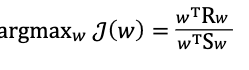
- maximize the ratio of the variance between classes to the one within the classes on the projected space
- it is a generalized eigenvalue problem (Rayleigh quotient)
- for 2 class cases, no need even to solve eigendecomposition
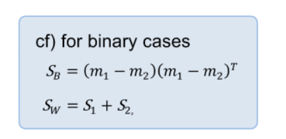
-
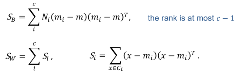
Multi-class case
- PCA and LDA
- Principal Component Analysis (PCA) and Linear Discriminant Analysis (LDA) are both dimensionality reduction techniques, but they have different objectives and are used in different contexts. Here are the key differences between PCA and LDA:
- Supervision:
- Objective:
- PCA: PCA aims to maximize the variance in the data. It identifies the directions (principal components) along which the data varies the most.
- LDA: LDA, on the other hand, aims to maximize the separation between classes. It identifies the directions that maximize the distance between the means of different classes while minimizing the spread (variance) within each class. - PCA: PCA is an unsupervised technique, meaning it does not take into account any class labels or information about the classes. - LDA: LDA is a supervised technique. It requires class labels for each data point to learn the linear combinations of features that best separate the classes.
- Objective:
- Application:
- PCA: PCA is often used for reducing the dimensionality of data when the goal is to capture the most important patterns or variability in the entire dataset, without specific regard to class labels.
- LDA: LDA is commonly employed in classification problems where the goal is to distinguish between different classes. It is used to find the linear combinations of features that are most informative for classification.
- Number of Components:
- PCA: In PCA, the number of principal components is determined by the number of features in the original data. It doesn’t consider class information.
- LDA: In LDA, the number of discriminant components is at most (c-1), where (c) is the number of classes. The maximum number of discriminant components is limited by the number of classes.
- Variance vs. Discrimination:
- PCA: PCA focuses on maximizing the total variance in the dataset. It is not concerned with class discrimination.
- LDA: LDA focuses on maximizing the ratio of between-class variance to within-class variance. It explicitly considers class information to find directions that maximize class separability.
- Assumptions:
- PCA: PCA assumes that the directions of maximum variance are the most important and informative directions in the data.
- LDA: LDA assumes that the data can be well-separated into classes, and it seeks the linear combinations of features that best discriminate between these classes.
In summary, PCA is primarily a dimensionality reduction technique that captures overall variance, while LDA is a supervised dimensionality reduction technique specifically designed for improving class separability in classification problems. The choice between PCA and LDA depends on the specific goals and nature of the data at hand.
- Supervision:
- cocktail party problem
- independent component analysis
- Independent Component Analysis (ICA) is a computational technique used for separating a multivariate signal into additive, independent components. The goal of ICA is to find a linear transformation of the data such that the resulting components are statistically as independent as possible. It is commonly applied in signal processing, neuroscience, and image analysis to identify and extract hidden factors contributing to observed data.
- a statistical problem
- to decompose given multivariate data into a linear sum of statistically independent components

- Maximum Likelihood Estimation (MLE):
- In the context of ICA, the observed data is assumed to be a linear combination of independent sources corrupted by noise. The demixing matrix is then estimated by maximizing the likelihood of the observed data given the model assumptions.
- The likelihood function involves the joint probability density function of the independent components. The demixing matrix that maximizes this likelihood is the one that effectively separates the sources.
- The optimization problem is often solved using algorithms like the FastICA algorithm, which seeks to find the demixing matrix that maximizes non-Gaussianity of the estimated sources.
- Super/Sub-Gaussianity:
- ICA relies on the assumption that the sources are statistically independent and have non-Gaussian distributions. Super-Gaussian sources have heavier tails than a Gaussian distribution, while sub-Gaussian sources have lighter tails.
- The non-Gaussianity assumption is crucial because Gaussian sources are not unique in ICA; any rotation or scaling of Gaussian sources can be considered a solution. Non-Gaussianity provides a measure of the independence of the estimated sources.
- The algorithms used in ICA often exploit measures of non-Gaussianity, such as kurtosis, to guide the separation process. Sources that are more non-Gaussian are considered more likely to be independent.
- nonnegative matrix factorization (NMF)
- constraint: W and H can not have negative value
- all basis vectors in NMF have localized features
- so both the basis and encodings are sparse
- the variability of X is generated by combining these different parts
- the basis vectors are like Lego blocks without subtraction
- and define a convex cone
- Non-negative Matrix Factorization (NMF) is a linear algebraic technique used for decomposing a non-negative matrix into two lower-rank non-negative matrices. It is particularly useful for analyzing non-negative data, such as images, documents, or audio signals. NMF has applications in diverse fields, including image processing, topic modeling, and source separation, where it helps extract meaningful and interpretable patterns from the data.
- representation: local vs. distributed
- support vector machines (SVMs) vs. artificial neural networks (ANNs)
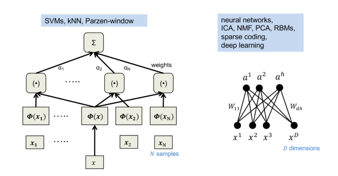
- representation: compact vs. sparse
- coding strategy
- sparseness
- equal response probability over the cells, low response probability for input