2023-HGU-ML Lecture 9. Nonlinear Dimension Reduction

Nonlinear Dimension Reduction

• Kernel machine and manifold learning
• extension of linear models with the kernel trick
  • kernel PCA
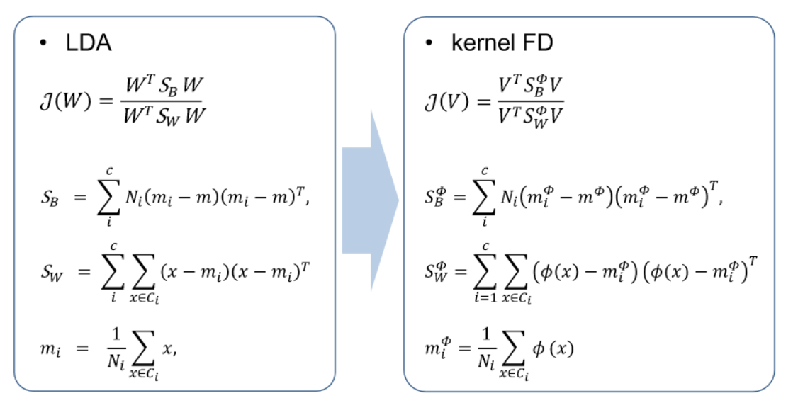
  • kernel Fisher discriminant (kernel FD)

  

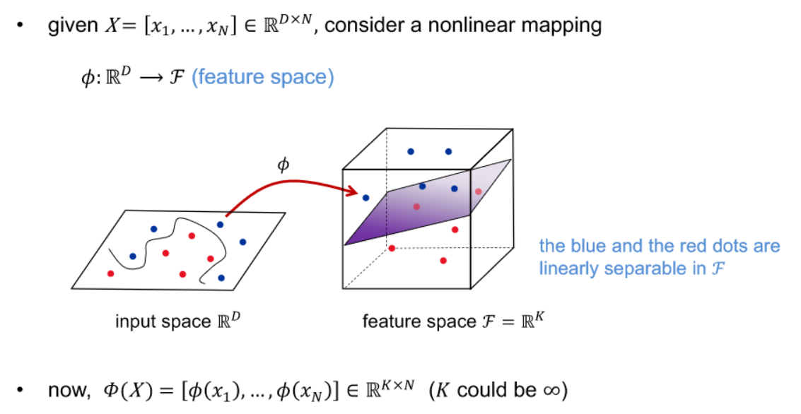
• Kernel trick
  • many ML algorithms are based on relations between samples’ inner product
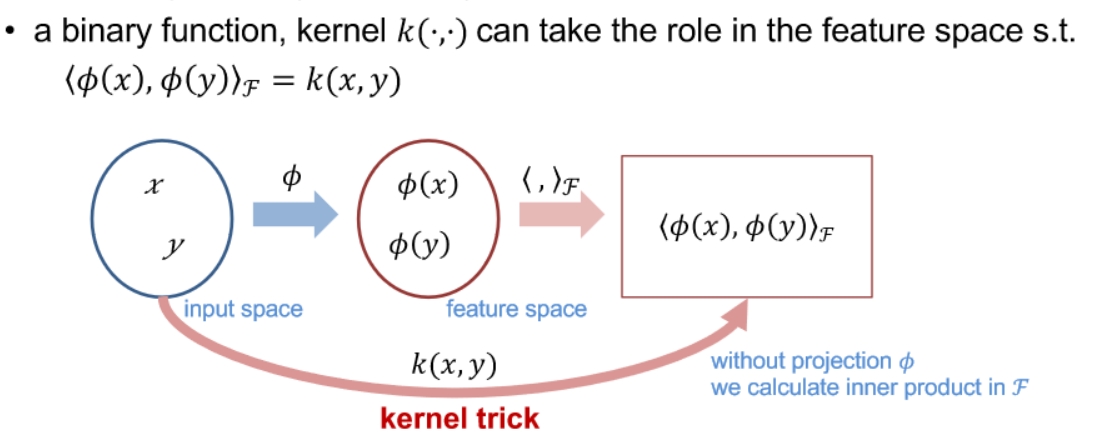
  • The kernel trick is a method in machine learning and support vector machines (SVMs) that allows the application of a linear algorithm in a high-dimensional feature space without explicitly calculating the transformed feature vectors. It is achieved by using a kernel function to compute the dot product between the transformed data points, which implicitly represents the higher-dimensional space. This technique is especially powerful when dealing with non-linearly separable data, enabling linear algorithms to effectively capture complex relationships by operating in a higher-dimensional space.

• Mercer’s theorem
  • any PSD kernel can be expressed as an inner product in some space
  • if a kernel function k(x, y) is positive semi definite(PSD), a PSD matrix can be eigen-decomposed

  

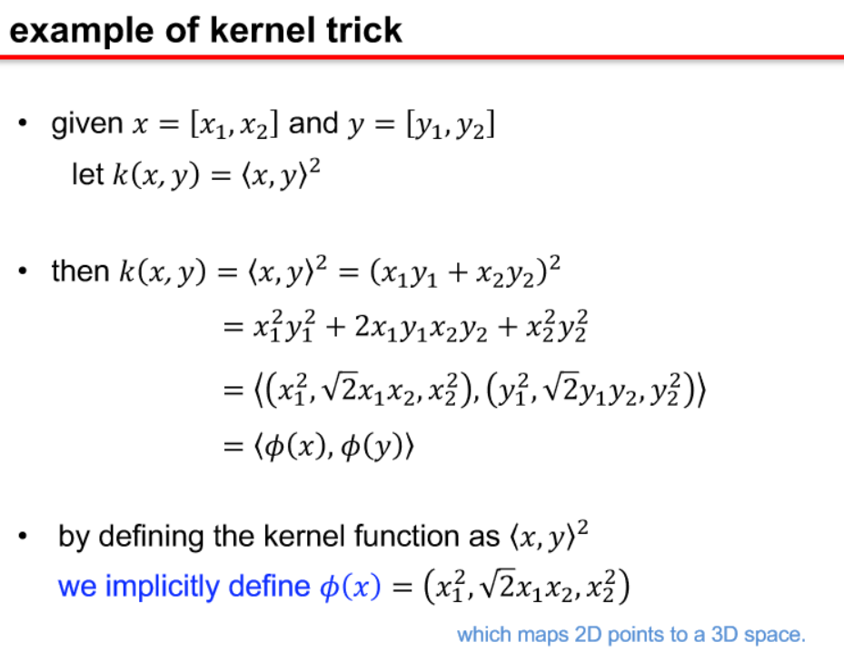
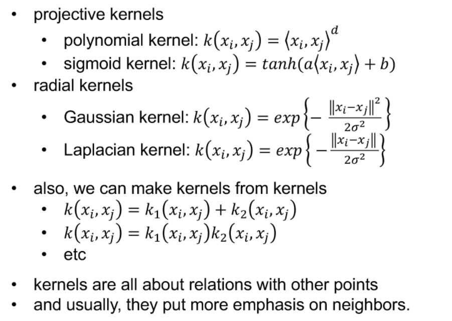
• kernel functions

  

• kernel PCA
  • Kernel Principal Component Analysis (Kernel PCA) is an extension of Principal Component Analysis (PCA) that utilizes the kernel trick to implicitly map input data into a higher-dimensional feature space. In traditional PCA, linear transformations are applied to find the principal components, but in Kernel PCA, a kernel function is used to capture non-linear relationships in the data. This allows Kernel PCA to uncover complex patterns and structures in high-dimensional spaces, making it particularly useful for tasks such as dimensionality reduction and non-linear feature extraction in machine learning.
• kernel FD
  • Kernel Fisher Discriminant (KFD) is an extension of Fisher’s Linear Discriminant Analysis (LDA) that incorporates the kernel trick to handle non-linearly separable data. Fisher’s LDA is a method used for finding linear combinations of features that best separate different classes in a dataset. KFD, through the use of a kernel function, allows this linear separation to be performed in a higher-dimensional space, enabling the discrimination of classes in a non-linear manner. Similar to Kernel PCA, Kernel Fisher Discriminant is particularly useful when dealing with complex, non-linear relationships in the data.

  

• manifold learning
  • usually, nonlinear dimension reduction
  • find the invariant property of a data set
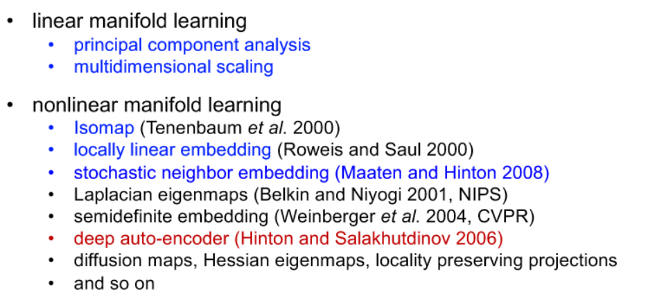
  • linear methods (PCA, LDA, ICA, NMF, etc)
  • nonlinear methods (kernel PCA, kernel FD, Isomap, LLE, etc)

  

• Isomap
  • manifold learning algorithms are to find the embedded manifold from data samples in a high dimensional space
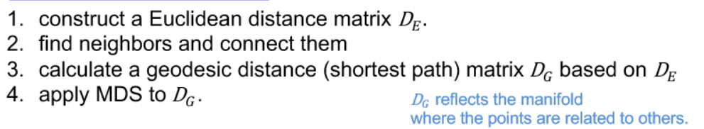
  • Isomap algorithm
    • uses geodesic distances on a neighborhood graph in the framework of MDS
    • https://en.wikipedia.org/wiki/Multidimensional_scaling

    

    • Deciding neighbors
      • KNN
      • epsilon neighborhood

• kernel Isomap

  

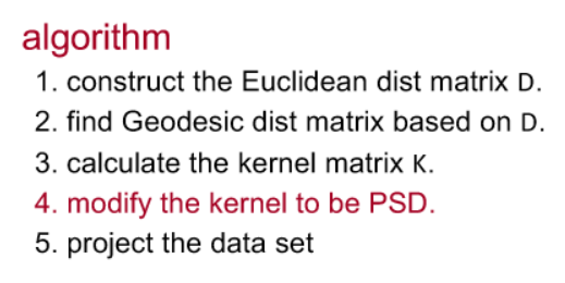
  • positive semi-definiteness
• locally linear embedding
  • keep the neighbors
  • Locally Linear Embedding (LLE) is a nonlinear dimensionality reduction algorithm that seeks to preserve the local linear relationships within a dataset. The key idea behind LLE is to represent each data point as a weighted linear combination of its neighbors, thereby capturing the local geometry of the data. Here’s a brief explanation of the LLE algorithm:
    1. Local Reconstruction:
       • For each data point in the high-dimensional space, LLE identifies its k nearest neighbors. These neighbors are the points that are most similar to the given point based on pairwise distances.
    2. Local Weight Optimization:
       • LLE then seeks to reconstruct the data point by finding the weights (coefficients) that best represent it as a linear combination of its neighbors. The reconstruction is performed in a way that minimizes the difference between the original point and its reconstruction.
    3. Global Embedding:
       • After obtaining the local linear representations for all data points, LLE seeks a lower-dimensional representation (embedding) for the entire dataset while preserving these local relationships. This is achieved by minimizing a cost function that enforces consistency in the local linear relationships across the entire dataset.
    4. Final Embedding:
       • The resulting lower-dimensional representation is obtained by stacking the embeddings of all data points. This representation captures the intrinsic geometry of the data, emphasizing the local linear relationships.
• Isomap and LLE
  • Isomap takes a global strategy, while LLE local
  • LLE analyzes local linear coefficients and reconstruction error
    • no need to solve large dynamic programming problems
    • related to spectral clustering
• stochastic neighbor embedding
  • probabilistically decides if points are neighbors to a given point
  • convert similarity into the probability
  • neighbors are selected probabilistically
  • use distances in a low dimensional space which define probabilities
  • compute KL divergence between the two probabilities
  • minimize KL with respect to yi
  • Stochastic Neighbor Embedding (SNE) is a dimensionality reduction technique that aims to capture the local and global structures of high-dimensional data in a lower-dimensional space. SNE is particularly effective at preserving pairwise similarities between data points, making it well-suited for visualization and exploration of complex datasets.
• t-SNE
  • a symmetrized version of SNE with t-Student instead of Gaussian
  • t-SNE (t-Distributed Stochastic Neighbor Embedding) is an extension of the original SNE (Stochastic Neighbor Embedding) algorithm designed to address some of its limitations. Both SNE and t-SNE are nonlinear dimensionality reduction techniques that focus on preserving pairwise similarities between data points.

• t-SNE and SNE

  Comparison:

  • Crowding Problem:
    • One of the main challenges with SNE is the crowding problem, where points in high-dimensional space are too close together and end up being crowded in the lower-dimensional space. t-SNE addresses this issue by using a heavy-tailed distribution, leading to better separation of clusters.
  • Preservation of Global Structure:
    • While SNE can struggle with preserving global structures, t-SNE is designed to perform better in this aspect. It is often more effective in revealing the overall structure of the data.
  • Computational Complexity:
    • t-SNE can be computationally more expensive than SNE, especially for large datasets, due to the need to compute and optimize the heavy-tailed distribution
  • https://woosikyang.github.io/first-post.html
• neural network approaches
  • weakness in manifold learning (kernel machine): it does not scale well with sample size. (scales quadratically with the size) the training data is referenced for test data
  • let’s get back to parametric models, especially neural networks
  • self organizing map
  • restricted Boltzmann machine
  • autoencoder (trained with backprop)